
KASY0 is a cluster supercomputer built primarily as a technology demonstration and experimental evaluation platform for Sparse Flat Neighborhood Networks (SFNNs). This page gives a good overview of KASY0's network: the world's first SFNN. Unrelated to the network, this page also briefly discusses an interesting problem involving alignment of 3DNow! instructions for decoding.
This is the primary reason we built KASY0: to use the world's first Sparse Flat Neighborhood Network. The network design is:
./KASY0 100 02010770 128 3 17 23
Seed was   1058580131
Pattern Generated: 1D torus +/- 1      offsets
Pattern Generated: 2D torus all of row and col ( 16,  8)
Pattern Generated: 3D torus all of row and col (  8,  4,  4)
Pattern Generated: bit-reversal
Pattern Generated: hypercube
PairCt =   1536, Min = 23, Avg =  24.00, Max = 25

Hit Control-D if there are no network configurations to load.

  1 network configuration(s) pre-loaded.  Generating 4095 more.

Starting full genetic search.
At gen start, net[bestpos].hist[0][0] = 4671
New best at generation         1:
  0:   0  15  16  31  32  47  48  63  64  79  80  95  96 111 112 120 121 122 123 124 125 126 127
  1:   0   1   2   3   4   5   6   7   8   9  10  11  12  13  14  15  24  40  56  72  88 104 120
  2:   7  23  39  55  71  87 103 112 113 114 115 116 117 118 119 120 121 122 123 124 125 126 127
  3:   2  10  18  26  33  34  35  37  42  43  44  45  46  50  58  66  74  82  90  98 106 114 122
  4:   5  13  21  29  37  45  53  61  69  77  81  83  84  85  86  89  92  93  94 101 109 117 125
  5:   1   9  17  25  33  41  49  57  64  65  67  68  70  73  75  76  78  81  89  97 105 113 121
  6:   4  12  16  18  19  20  22  23  27  28  30  36  44  52  60  68  76  84  92 100 108 116 124
  7:   3  11  19  27  35  43  51  59  67  75  83  91  96  98  99 102 103 104 107 109 110 115 123
  8:   6  14  22  30  38  46  48  50  53  54  55  56  59  60  62  70  78  86  94 102 110 118 126
  9:  32  36  38  39  40  41  47  48  49  50  51  52  53  54  55  56  57  58  59  60  61  62  63
 10:   2  32  33  34  35  36  37  38  39  40  41  42  43  44  45  46  47  69  71  72  73  74  79
 11:  64  65  66  67  68  69  70  71  72  74  75  76  77  78  79  80  82  87  88  90  91  93  95
 12:   5  17  20  21  24  26  29  31  80  81  82  83  84  85  86  87  88  89  90  91  92  94  95
 13:   7   8  15  16  17  18  19  20  21  22  23  24  25  26  27  28  29  30  31 100 101 105 111
 14:  66  73  77  85  96  97  98  99 100 101 102 103 104 105 106 107 108 109 110 111 112 117 119
 15:  49  51  52  54  57  58  61  62  63  65  93  97  99 106 107 108 113 114 115 116 118 119 127
 16:   0   1   3   4   6   8   9  10  11  12  13  14  25  28  34  42
 17.
NICs/PC: 0[     0] 1[     0] 2[     0] 3[   128]
Dist[0]: 0[  4671] 1[  2769] 2[   665] 3[    23]
Dist[1]: 0[     0] 1[   957] 2[   556] 3[    23]
Above has Quality  99023211
The lines starting with a number followed by ":" specify the actual wiring pattern; the first number is the switch number, the remaining numbers on each line are the node numbers connected to that switch.
Another innovative aspect of KASY0's network is the physical layout. Last year, we began developing software tools that could help design optimized physical layouts. In general, as the node count gets large, spiral rack patterns become the single-story winner; KASY0's 6 racks are not enough to be obvious as a spiral, but look more like a slightly deformed circle. Switches are distributed throughout the PC racks to take advantage of wiring locality. One might think that SFNNs need to sacrifice wiring locality properties to achieve their single-switch latency for a wide range of communication patterns, but this is not the case. If physically laid out in the obvious way, 282 of KASY0's 384 network cables would cross racks; a newly developed GA found a physical arrangement that reduces the crossing count to 159 cables, and this is pattern that we used:
Rack 0:
 Switches: 4 11 12
 PCs: 66  5 21 29 69 77 80 81 82 83 84 85 86 87 88 89 90 91 92 93 94 95
Rack 1:
 Switches: 8 9 15
 PCs: 97 108 116  38 48 49 50 51 52 53 55 56 57 58 59 60 61 63 118  54 62
Rack 2:
 Switches: 2 7 14
 PCs: 7 67 73 113 121 125 126  96 98 99 102 104 107 109 110 112 115 117 119 123  103
Rack 3:
 Switches: 0 6 13
 PCs: 26 47 68 76 101 120 122 127  15 18 19 20 22 23 27 28 30 31 100 111 124  16
Rack 4:
 Switches: 1 5 16
 PCs: 17 24 64 65 70 75 78 105  0 3 4 6 8 10 11 12 13 14 25  1 9
Rack 5:
 Switches: 3 10
 PCs: 32 36 39 40 41 71 72 79 106 114  2 33 34 35 37 42 43 44 45 46 74
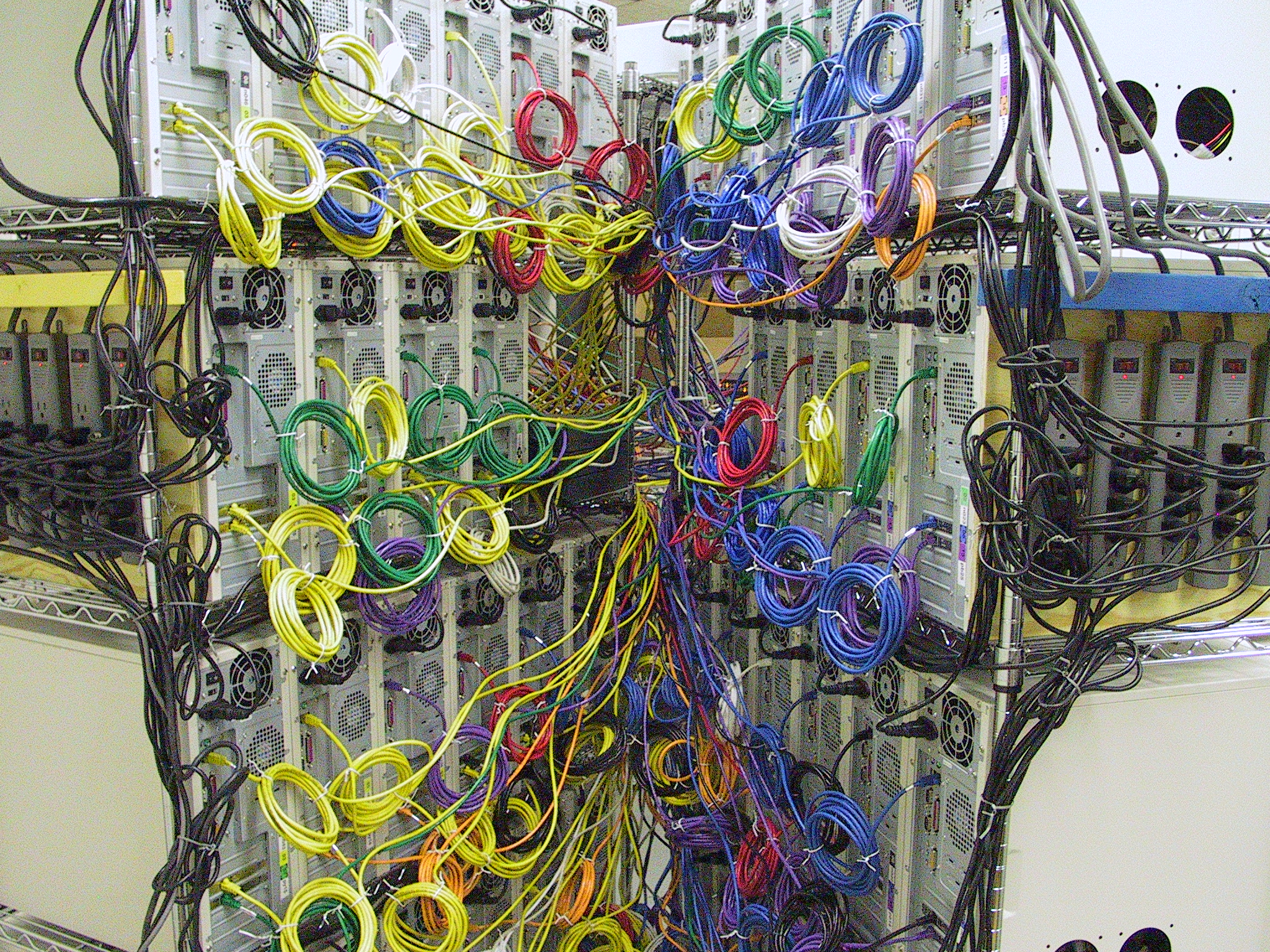
The following photo shows how we color-coordinated the rack color markings with the switch cable colors to make the wiring and identification of logical-to-physical mappings relatively straightforward. The image shows the "yellow rack" and the "blue rack" -- notice that switches are positioned so that the switches with yellow-based colors (yellow and yellow+stripe) are on the yellow rack and the blue-based colors (blue, blue+stripe, and purple) are on the blue rack. Thus, minimizing physical wiring across racks also maximizes the "sameness" of the cable colors within each rack; cables to switches on other racks stand-out against the dominant rack color.
To facilitate identifying nodes, each node has two separate names:
It turns out that the same concepts are useful in numbering switches.
That's all well and good, but how does this all come together? Well, take a look at KASY0-labels.html; this is the HTML source for the automatically-generated node labels using the above scheme.
Use of 3DNow! for technical computing is not really a new technology -- although it was new when we used it on KLAT2 -- but KASY0 has a new implementation of the SGEMM routine for Automatically Tuned Linear Algebra Software (ATLAS) that we have tuned for maximum possible 3DNow! performance. The new version is significantly faster than both the version we developed for KLAT2 and the version currently packaged with ATLAS. Running on a single node, the new version achieves between 87% and 97% (depending on what's cached before it's invoked ;-) of the theoretical peak floating point performance of an Athlon XP 2600+.
The primary new trick involves careful alignment of groups of 3 instructions on 16-byte boundaries to maximize instruction decode performance. Initial alignment for a block of code can be accomplished using an alignment directive. To maintain alignment for groups of 3 DirectPath-decoded instructions, aside from careful choice of instruction addressing modes (which implies instruction length), most instructions can be made a byte longer using the otherwise harmless REP prefix byte, 0xf3. The alignment issue is not fitting as much as possible into 8- or 16-byte chunks (as popularly believed); it is literally having groups of 3 instructions that are able to be decoded as a set arranged so that the sequence cleanly aligns with 16-byte (or pairs of 8-byte) boundaries. Tim Mattox, who implemented these changes, suggests it is best to view the Athlon as a 3-wide VLIW with 16-byte instruction words. The fail-safe-VLIW model also yields a more accurate view of the dynamic scheduling inside the Athlon. Anyone want to make GCC understand that? Well, at least our new SGEMM will be incorporated in the standard ATLAS distribution....
BTW, this alignment constraint is an Athlon thing: the new Opteron and Athlon 64 processors have significantly different decoder structures, which have less-obtrusive 16-byte alignment issues.
![]() The only thing set in stone is our name.
The only thing set in stone is our name.